This is the continuation of a project where I explore and visualize data from OKCupid.
You also might want to check out Dating Pools using K-Means Clustering, which also uses our OKCupid data.
Work Skills showcased in this article:
- Hyperparameter Tuning of Machine Learning Models using scikit-learn
- Machine Learning Model Evaluation and Comparison
- Analyzing Top Predictors used by a trained Model
- Visualization of Machine Learning Tuning, Training, and Evaluation using Plotly
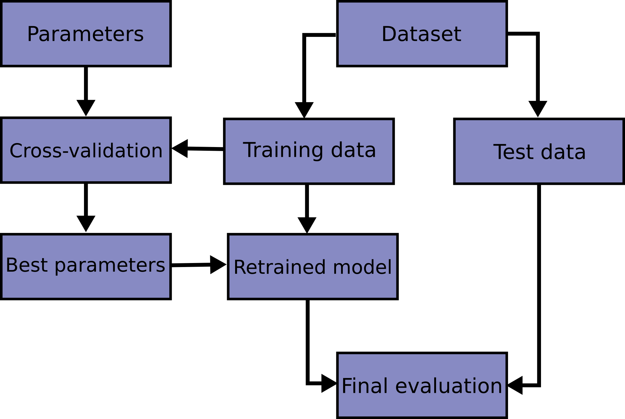
Block Diagram of Model Tuning and Evaluation
The diagram below comes from scikitlearn docs. This is the procedure that we will follow. The left section outlines the model parameter tuning process. The right section outlines the model test setup and evaluation process.
#Configure if model parameter tuning will be executed:
execute_dt_search = True
execute_rf_search = True
execute_lr_search = True
Load data
import pandas as pd
from scipy.sparse import coo_matrix

df = pd.read_csv('ml_ready_data.csv')
df.info()
<class 'pandas.core.frame.DataFrame'>
RangeIndex: 59811 entries, 0 to 59810
Columns: 738 entries, Unnamed: 0 to speaks_yiddish (poorly)
dtypes: int64(728), object(10)
memory usage: 336.8+ MB
Separate Features and Labels
def feature_selection_to_list(df, cat_selection, numeric_selection):
    categorical_feats = []
    for each in cat_selection:
        categorical_feats = categorical_feats + df.loc[:, df.columns.str.startswith(each)].columns.to_list()
    return categorical_feats + numeric_selection

cat_selection = ['body_type', 'drinks', 'drugs', 'education', 'job', 'orientation',
                'smokes', 'status', 'diet_adherence', 'diet_type', 'last_online',
                'offspring_want', 'offspring_attitude', 'religion_type', 'religion_attitude',
                'sign_type', 'sign_attitude', 'dog_preference', 'cat_preference', 'has_dogs',
                'has_cats', 'ethnicity', 'speaks']
numeric_selection = ['age', 'height']
feature_selection = feature_selection_to_list(df, cat_selection, numeric_selection)

predictors = df[feature_selection]
predictor_legend = ['Male Predictor', 'Female Predictor']
labels = df.sex
Import Libraries
from sklearn.pipeline import Pipeline
from sklearn.linear_model import LogisticRegression
from sklearn.model_selection import GridSearchCV
from sklearn.preprocessing import StandardScaler
from sklearn.tree import DecisionTreeClassifier
from sklearn.ensemble import RandomForestClassifier
from sklearn.model_selection import cross_val_score
import plotly.express as px
import numpy as np
import time
Model Parameter Tuning
Some explanations are necessary before you dive in. GridSearchCV is a function for repeatedly building a model using different combinations of a set of specified parameter values. In addition, GridsearchCV also makes use of StratifiedKfold, to report a model score. It is your decision which evaluation metric to use as the score, but by default accuracy is used. If you do not pass an argument to the cv parameter of your GridSearchCV function, it uses k=5, or 5-fold cross validation, by default. However, if you want to specify the parameters, or choose a different validator such as RepeatStratifiedKfold, then you pass a validator function, complete with specified parameters, as the argument of cv.
By not passing an argument below, the default cv is used.
It’s a good idea to reconsider what the project objective was. The original goal was “Use Machine Learning to predict gender”. In this case we don’t want the model to discriminate against gender. As much as possible we want it to perform equally well for either class. Which is why the metric we will use as the model score for GridSearchCV will be accuracy, its default.
#Log Tuning Time
start = time.time()
Logistic Regression Model
Tuning (Parameter = C)
C represents regularization strength.
if execute_lr_search:
    model = GridSearchCV(estimator=LogisticRegression(),
                 param_grid={'C': list(range(1, 11))})
    pipe_lr = Pipeline([('scaler', StandardScaler()), ('LogisticRegression', model)])
    pipe_lr.fit(predictors, labels)
Results
if execute_lr_search:
    print("The best score is: {}".format(pipe_lr['LogisticRegression'].best_score_))
    print("The best parameters are: {}".format(pipe_lr['LogisticRegression'].best_params_))
    fig = px.scatter(pd.DataFrame(pipe_lr['LogisticRegression'].cv_results_), x='param_C', y='mean_test_score', title = 'Different values of C')
    fig.data[0].update(mode='markers+lines')
    fig.show()
    fig.write_html("lrsearch.html")
The best score is: 0.8885489343130564
The best parameters are: {'C': 1}
Decision Tree Model
Tuning (Parameter = max_depth)
Max Tree Depth
if execute_dt_search:
    model = GridSearchCV(estimator=DecisionTreeClassifier(),
                 param_grid={'max_depth': list(range(3, 100))})
    pipe_dt = Pipeline([('scaler', StandardScaler()), ('DecisionTreeClassifier', model)])
    pipe_dt.fit(predictors, labels)
Results
if execute_dt_search:
    print(pipe_dt['DecisionTreeClassifier'].best_score_)
    print(pipe_dt['DecisionTreeClassifier'].best_params_)
    fig = px.scatter(pd.DataFrame(pipe_dt['DecisionTreeClassifier'].cv_results_), x='param_max_depth', y='mean_test_score', title = 'Different tree depths')
    fig.data[0].update(mode='markers+lines')
    fig.show()
    fig.write_html("Decision_tree_depths.html")
Random Forest Model
Tuning (Parameters = max_depth, n_estimators)
Max Tree Depth and Number of Trees in the Forest
if execute_rf_search:
    model = GridSearchCV(estimator=RandomForestClassifier(),
                 param_grid={'max_depth': list(range(6, 40)), 'n_estimators': [150, 180, 300]})
    pipe_rf = Pipeline([('scaler', StandardScaler()), ('rfc', model)])
    pipe_rf.fit(predictors, labels)
Results
if execute_rf_search:
    print(pipe_rf['rfc'].best_score_)
    print(pipe_rf['rfc'].best_params_)
    fig = px.scatter_3d(pd.DataFrame(pipe_rf['rfc'].cv_results_),
                        x='param_max_depth',
                        y = 'param_n_estimators',
                        z='mean_test_score',
                        color = 'mean_test_score',
                        color_continuous_scale = 'Viridis',
                        title = 'Different Random Forest Parameters')
    fig.show()
    fig.write_html("Random_forest_grid_crossval.html")
The 3D Scatter plot can be rotated, panned, and zoomed.
Note that with the Random Forest we are still gaining better performance with higher max depth, unlike with the Decision Tree which completely drops after peaking at depth = 7.
Tuning Duration
end = time.time()
duration = round(end-start, 2)
print("Time to tune 3 models was: " + str(duration) + " secs")
Time to tune 3 models was: 24837.2 secs
It took 7 hours to tune the parameters of the three models! Majority of the tuning time was taken up by the Random Forest.
Dataset splitting
Let’s set aside our test and train sets.
from sklearn.model_selection import train_test_split

X_train, X_test, y_train, y_test = train_test_split(predictors, labels, test_size=0.2, random_state=1)
Retraining Models using Optimized Parameters
start = time.time()

model = LogisticRegression()
pipe_lr = Pipeline([('scaler', StandardScaler()), ('LogisticRegression', model)])
model = DecisionTreeClassifier(max_depth = 7)
pipe_dt = Pipeline([('scaler', StandardScaler()), ('DecisionTreeClassifier', model)])
model = RandomForestClassifier(max_depth = 34, n_estimators = 300)
pipe_rf = Pipeline([('scaler', StandardScaler()), ('RandomForestClassifier', model)])

trained_pipe_lr = pipe_lr.fit(X_train, y_train)
trained_pipe_dt = pipe_dt.fit(X_train, y_train)
trained_pipe_rf = pipe_rf.fit(X_train, y_train)

end = time.time()
duration = round(end-start, 2)
print("Time to train 3 models was: " + str(duration) + " secs")
Time to train 3 models was: 73.11 secs
Model Evaluation and Comparison
lr_predictions = trained_pipe_lr.predict(X_test)
dt_predictions = trained_pipe_dt.predict(X_test)
rf_predictions = trained_pipe_rf.predict(X_test)

model_accuracy_dict = {}
model_list = [trained_pipe_lr, trained_pipe_dt, trained_pipe_rf]
model_names = ['LogisticRegression', 'DecisionTreeClassifier', 'RandomForestClassifier']
for model, name in zip(model_list, model_names):
    test_score = model.score(X_test, y_test)
    model_accuracy_dict[name] = test_score
accuracy_df = pd.DataFrame(model_accuracy_dict, index = ["Accuracy"])
fig = px.bar(accuracy_df.transpose(), y=model_names, x = "Accuracy", orientation = 'h')
fig.update_xaxes(range=(0.84, 0.9))
fig.update_yaxes(categoryorder = "total ascending")
fig.update_traces(texttemplate='%{value:.3f}', textposition = 'outside')
fig.update_layout(title="Accuracy of Different Models", yaxis_title="Model",)
fig.show()
fig.write_html("modelaccuracy.html")
This chart shows us the different model accuracies. What it does not tell us is how well the models performed between Males and Females. For that information we need to look at a Confusion Matrix.
from sklearn.metrics import confusion_matrix

confusion_matrices = []
for name, predictions in zip(model_names, [lr_predictions, dt_predictions, rf_predictions]):
    confusion_df = pd.DataFrame(confusion_matrix(y_test, predictions, normalize = 'true'),
                                columns = ['pred_Female', 'pred_Male'],
                                index = ['actual_Female', 'actual_Male'])
    confusion_df = confusion_df.transpose()
    confusion_df['Model'] = name
    confusion_df['actual_Female'] = confusion_df['actual_Female']*100
    confusion_df['actual_Male'] = confusion_df['actual_Male']*100
    confusion_matrices.append(confusion_df)
confusion_df = pd.concat([matrix for matrix in confusion_matrices])
confusion_df
Confusion Matrix
| actual_Female | actual_Male | Model | |
|---|---|---|---|
| pred_Female | 85.5861 | 8.36937 | LogisticRegression |
| pred_Male | 14.4139 | 91.6306 | LogisticRegression |
| pred_Female | 80.7468 | 9.06682 | DecisionTreeClassifier |
| pred_Male | 19.2532 | 90.9332 | DecisionTreeClassifier |
| pred_Female | 83.2708 | 7.46269 | RandomForestClassifier |
| pred_Male | 16.7292 | 92.5373 | RandomForestClassifier |
The Confusion Matrix is a cross-tabulation between the actual gender of our users and the model’s predicted gender of our users. In this case we produced a confusion matrix where the values are percentages, but you can also make one that shows counts.
import plotly.graph_objects as go

fig = go.Figure(data = [
    go.Bar(
        x=confusion_df.actual_Male.loc['pred_Male'],
        y=confusion_df.Model.loc['pred_Male'],
        name = 'Correctly Classified Males',
        orientation='h',
        offsetgroup = 0,
        texttemplate = '%{value:.1f}%',
        textposition = 'inside',
        hoverinfo = 'none'
    ),
    go.Bar(
        x=confusion_df.actual_Male.loc['pred_Female'],
        y=confusion_df.Model.loc['pred_Female'],
        name = 'Misclassified Males',
        orientation='h',
        offsetgroup = 0,
        base = [each for each in confusion_df.actual_Male.loc['pred_Male']],
        texttemplate = '%{value:.1f}%',
        textposition = 'inside',
        hoverinfo = 'none'
    ),
    go.Bar(
        x=confusion_df.actual_Female.loc['pred_Female'],
        y=confusion_df.Model.loc['pred_Female'],
        name = 'Correctly Classified Females',
        orientation='h',
        offsetgroup = 1,
        texttemplate = '%{value:.1f}%',
        textposition = 'inside',
        hoverinfo = 'none'
    ),
    go.Bar(
        x=confusion_df.actual_Female.loc['pred_Male'],
        y=confusion_df.Model.loc['pred_Male'],
        name = 'Misclassified Females',
        orientation='h',
        offsetgroup = 1,
        base = [each for each in confusion_df.actual_Female.loc['pred_Female']],
        texttemplate = '%{value:.1f}%',
        textposition = 'inside',
        hoverinfo = 'none'
    ),
                ],
                layout=go.Layout(
                    title="Male & Female Class Predictions per Model",
                    yaxis_title="Model",
                    xaxis_title = "Percentage"
                )
               )
fig.update_xaxes(range=(0, 100))
fig.show()
fig.write_html("confusionbars.html")
The plot may be zoomed in on the rightmost region, in order to further highlight differences.
In all cases the models perform better at classifying males than females. In the best case, the logistic regression model, men are classified 6.77% times better than women. A consequence of either training on a male-skewed dataset or not having enough reliable features that allow the model to confidently classify women (or both).
This is not without consequence in the real world. In the documentary “Coded Bias”, during a senate hearing, Alexandra Ocasio-Cortez questions Joy Buolamwini. Here is a selected excerpt:
AOC: “What demographic is it [AI models] mostly effective on?”
JB: “White Men”
AOC: “And who are the primary engineers and designers of these algorithms?”
JB: “Definitely white men”
Despite the oral exchange above, it’s possible to make a biased AI model without being a “white man”. You could be an ML engineer who failed to properly evaluate the performance of your model at identifying all class labels. This issue has already entered the mainstream social and political spheres.
Examination of Predictor Weights and Importances
predictor_legend = ['Male Predictor', 'Female Predictor']
fig = px.bar(
        y=predictors.columns,
        x=abs(trained_pipe_lr['LogisticRegression'].coef_[0]),
        color=[predictor_legend[0] if c > 0 else predictor_legend[1] for c in trained_pipe_lr['LogisticRegression'].coef_[0]],
        color_discrete_sequence=['red', 'blue'],
        labels=dict(x='Predictor', y='Weight/Importance'),
        title='Top 20 Predictors of the Logistic Regression Model',
    )
fig.update_yaxes(categoryorder = "total ascending", range=(len(predictors.columns) - 20.6, len(predictors.columns)))
fig.show()
fig.write_html("lrpreds.html")

fig = px.bar(
        y=predictors.columns,
        x=trained_pipe_dt['DecisionTreeClassifier'].feature_importances_,
        labels=dict(x='Predictor', y='Weight/Importance'),
        title='Top 20 Predictors of the Decision Tree Model',
    )
fig.update_yaxes(categoryorder = "total ascending", range=(len(predictors.columns) - 20.6, len(predictors.columns)))
fig.show()
fig.write_html("dtpreds.html")

fig = px.bar(
        y=predictors.columns,
        x=trained_pipe_rf['RandomForestClassifier'].feature_importances_,
        labels=dict(x='Predictor', y='Weight/Importance'),
        title='Top 20 Predictors of the Random Forest Model',
    )
fig.update_yaxes(categoryorder = "total ascending", range=(len(predictors.columns) - 20.6, len(predictors.columns)))
fig.show()
fig.write_html("rfpreds.html")
For all models, height and body_type_curvy are our top predictors. Probably because men are taller than women on average, and perhaps men are not likely to describe themselves as curvy whereas women are. It is interesting to see that after the top two predictors, there is a different order of feature importances for the random forest compared to the other models.
With Logistic Regression we can conveniently see which features were more useful for predicting class (male or female) because we have negative and positive weight coefficients, unlike with the Random Forest and Decision Tree.
Next Steps
Although not presented here, most likely, because the age distribution is skewed towards the young, the model is more effective at classifying young people than old people. One way to alleviate this is to apply a power transform to the age distribution, which makes it more like a normal distribution, before training (you will also have to apply the same transform to the test set before predicting). Then you will have to evaluate the model’s performance with young vs old subsets of our data.
Model evaluation can still be taken steps further. In scikit learn there is an example of applying frequentist and bayesian statistical approaches to more definitively make model comparisons.
Now that you know how to evaluate a model, the challenge is to learn how to improve model performance. Not just in general, but to be fair at identifying all classes. You will rarely ever have a dataset that is perfectly balanced.